可以试试这个
https://github.com/gxywy/rl-plotter

Installation from PIP

pip install rl_plotter

from source

python setup.py install

Usage
Add our logger (compatible with OpenAI-baseline) in your code or just use OpenAI-baseline bench.Monitor (recommended):

from baselines import bench
env = bench.Monitor(env, log_dir)

After the training or when you are training your agent, you can plot the learning curves in this way:

switch to log directory (default: ./)

run command to plot:

rl_plotter --save --show
more general commands in practice:

rl_plotter --save --show --avg_group --shaded_std
rl_plotter --save --show --avg_group --shaded_std --time
rl_plotter --save --show --avg_group --shaded_std --shaded_err

for help:

rl_plotter --help
and you can find parameters to custom the style of your curves.

optional arguments:
-h, --help show this help message and exit
--fig_length matplotlib figure length (default: 6)
--fig_width matplotlib figure width (default: 6)
--style matplotlib figure style (default: seaborn)
--title matplotlib figure title (default: None)
--xlabel matplotlib figure xlabel
--xkey x-axis key in csv file (default: l)
--ykey y-axis key in csv file (default: r)
--ylabel matplotlib figure ylabel
--smooth smooth radius of y axis (default: 10)
--resample if not zero, size of the uniform grid in x direction
to resample onto. Resampling is performed via
symmetric EMA smoothing (see the docstring for
symmetric_ema). Default is zero (no resampling). Note
that if average_group is True, resampling is
necessary; in that case, default value is 512.
(default: 512)
--smooth_step when resampling (i.e. when resample > 0 or
average_group is True), use this EMA decay parameter
(in units of the new grid step). See docstrings for
decay_steps in symmetric_ema or one_sided_ema functions.
(default: 1.0)
--avg_group average the curves in the same group and plot the mean
--shaded_std shaded region corresponding to standard deviation of the group
--shaded_err shaded region corresponding to error in mean estimate of the group
--legend_loc location of legend
--legend_outside place the legend outside of the figure
--no_legend_group_num don't show num of group in legend
--time enable this will set x_key to t, and activate parameters about time
--time_unit parameters about time, x axis time unit (default: h)
--time_interval parameters about time, x axis time interval (default: 1)
--xformat x-axis format
--xlim x-axis limitation (default: None)
--log_dir log dir (default: ./)
--filename csv filename
--show show figure
--save save figure
--dpi figure dpi (default: 400)
finally, the learning curves looks like this:

2 个月 后
3 个月 后
4 个月 后

panchao12345 代表置信区间或者叫误差区间,因为在x轴上每个小小的区间段,有很多个episode rewards,所以有一个上下波动的范围,画图软件会自动帮你估计出中间值的位置,也就是那条线的位置。

  • Yhp 回复了此帖
    8 天 后

    bug404 您好,这个seaborn如何根据tensorboard文件绘制出类似上面的曲线图呢


    [未知] 还是不太会画,能否指导一下呢

    [未知] 我画不出这种效果,能否指导一下呢

      6 个月 后
      9 天 后

      请问我用了seaborn画图,数据是由三组随机种子生成的,为什么画出来的图没有阴影啊?好像都叠在了一起

        5 个月 后

        想问怎么用rl_plotter绘制已经存在的csv文件,绘制成文章中图的样子?

        • aoao 回复了此帖
          3 个月 后
          1 年 后

          wagh311

          import os
          import numpy as np
          import matplotlib.pyplot as plt
          import pandas as pd
          from statsmodels.nonparametric.smoothers_lowess import lowess
          
          def loess_smooth(data, frac=0.035):
              x = np.arange(len(data))
              smooth_result = lowess(data, x, frac=frac)
              return smooth_result[:, 1]
          
          # 生成示例数据
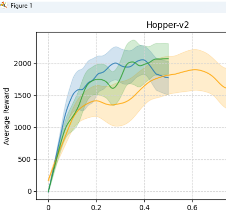
          environments = ["HalfCheetah-v2", "Hopper-v2", "Swimmer-v2", "Walker2d-v2"]
          algorithms = ["PPO", "SAC", "DPPO"]
          
          # 设置文件路径列表
          file_paths = {
              "HalfCheetah-v2": ['Half1.csv', 'Half2.csv', 'Half3.csv'],     # 例如:Half.csv中包含seed1,seed2,seed3三列数据(奖励)
              "Hopper-v2": ['Hopper1.csv', 'Hopper2.csv', 'Hopper3.csv'],
              "Swimmer-v2": ['Swimmer1.csv', 'Swimme2.csv', 'Swimmer3.csv'],
              "Walker2d-v2": ['Walker1.csv', 'Walker2.csv', 'Walker3.csv']
          }
          
          # 创建一个2x2的子图布局
          fig, axs = plt.subplots(2, 2, figsize=(12, 8))
          
          # 创建颜色映射
          color_map = {alg: plt.cm.tab10(i) for i, alg in enumerate(algorithms)}
          
          # 模拟一些数据,以便演示
          for i, env in enumerate(environments):
              ax = axs[i // 2, i % 2]
          
              # 存储当前环境的算法标签
              env_handles = []
              env_labels = []
          
              for file_path, algorithm in zip(file_paths[env], algorithms):
                  df = pd.read_csv(file_path)
                  reward_data = [df[col].tolist() for col in df.columns]
                  mean_rewards = np.mean(reward_data, axis=0)
                  std_rewards = np.std(reward_data, axis=0)
          
                  # 对均值进行Loess平滑处理
                  smoothed_mean_rewards = loess_smooth(mean_rewards, frac=0.035)
          
                  # 对标准差进行Loess平滑处理
                  smoothed_std_rewards = loess_smooth(std_rewards, frac=0.035)
          
                  # 特殊处理 PPO 的颜色
                  if algorithm == "PPO":
                      color = 'orange'
                  else:
                      color = color_map[algorithm]
          
                  # 绘制平滑处理后的奖励函数图
                  line, = ax.plot(smoothed_mean_rewards, label=f'{algorithm}', alpha=0.8, color=color)
                  ax.fill_between(range(len(smoothed_mean_rewards)), smoothed_mean_rewards - smoothed_std_rewards,
                                  smoothed_mean_rewards + smoothed_std_rewards, alpha=0.2, color=color)
          
                  # 存储当前算法的标签和线条
                  env_handles.append(line)
                  env_labels.append(f'{algorithm}')
          
          
              ax.set_title(f"{env}")
              ax.set_xlabel('Time Steps(1e6)')
              ax.set_ylabel('Average Reward')
          
              # 在当前子图中手动创建图例
              ax.legend(handles=env_handles, labels=env_labels, loc='lower right')
          
              # 添加浅灰色虚线网格线
              ax.grid(True, linestyle='--', color='lightgrey')
          
              # # 修改横坐标
              labels=["0",'0','0.2','0.4','0.6','0.8','1M']
              # total_steps = len(smoothed_mean_rewards)  # 获取总步数
              # steps_in_millions = np.linspace(0, total_steps - 1, 6) / 1e6  # 将总步数分割为6个点
              ax.set_xticklabels(labels)
          
          
          # 调整布局以防止标题重叠
          plt.tight_layout()
          # 保存图为PDF文件(dpi=600)
          plt.savefig('multi-result.pdf', format='pdf', dpi=600)
          
          # 显示图形
          plt.show()
            18 天 后
            说点什么吧...
            Document